Of VJPs and JVPs

Suppose that we have a function \(f: \R^{n} \to \R^{m}\), which maps an \(n\)-dimensional input \(\rvx \in \R^{n}\) to an \(m\)-dimensional output \(\rvy \in \R^{m}\). 0: In machine learning, we often work with parametric functions: \(f(\rvx; \vtheta)\), in which case we might also be more interested in differentiating wrt. these parameters \(\vtheta\) than the data \(\rvx\). For clarity, we will stick to the first case for now, however in a later section we will see how we can recover a function in \(\vtheta\) only by essentially averaging out the data term. For now, you could think of ‘partially applying’ an input data point—resulting in a new function \(f_{\rvx}: \R^{n} \to \R^{m}\) where we have assumed \(\vtheta \in \R^{n}\). ^0[0]

One way to view this function is as a column vector of \(m\) scalar-valued functions stacked one on top of each other:

The Jacobian matrix \(\rmJ\) of \(f\) is an \(m \times n\) matrix, where each row contains the gradient of the \(i\)‘th ‘scalar function’ wrt the inputs \(\rvx\), \(\nabla_{\rvx}f_{i}(\rvx)\):

\[\rmJ = \begin{bmatrix} \hrule \nabla_{\rvx}f_{1}(\rvx) \hrule \\ \hrule \nabla_{\rvx}f_{2}(\rvx) \hrule \\ \vdots \\ \hrule \nabla_{\rvx}f_{m}(\rvx) \hrule \\ \end{bmatrix} = \begin{bmatrix} \frac{\partial \ervy_{1}}{\partial \ervx_{1}} & \frac{\partial \ervy_{1}}{\partial \ervx_{2}} & \cdots & \frac{\partial \ervy_{1}}{\partial \ervx_{n}} \\ \vdots & \vdots & \ddots & \vdots \\ \frac{\partial \ervy_{m}}{\partial \ervx_{1}} & \frac{\partial \ervy_{m}}{\partial \ervx_{2}} & \cdots & \frac{\partial \ervy_{m}}{\partial \ervx_{n}} \end{bmatrix}. \]

More generally, the \(i, j\)-th entry of \(\rmJ\) contains the partial derivative of the \(i\)th output with respect to the \(j\)th input.

At risk of stating the obvious, the vector-Jacobian product (VJP) is the left-multiplication of the Jacobian by some vector, while the Jacobian-vector product (JVP) is the right-multiplication of the Jacobian by an appropriately shaped vector. Here are the definitions with a bit more detail:

Similarly, for the JVP

Note that the JVP really just corresponds to a first-order Taylor approximation to the function \(f\). If \(f\) is differentiable at some point \(\rvx_{0}\), then we can approximate it as:

\[f(\rvx) = f(\rvx_{0}) + \rmJ(\rvx - \rvx_{0}) + o(\Vert \rvx - \rvx_{0}\Vert), \]

where we use the little-o notation to denote that the remainder goes to \(0\) faster than \(\Vert \rvx - \rvx_{0}\Vert\) as \(\rvx \to \rvx_{0}\). We often refer to this as the linearization of \(f\).

A Concrete Example

Let’s consider a very simple function with \(n=3\) inputs and \(m=2\) outputs to illustrate what’s going on:

\[f(\rvx) \doteq \begin{bmatrix}\ervx_{1}^{2} + \ervx_{2} + \ervx_{3} \\ \ervx_{1} - \ervx_{2} + \ervx_{3} \end{bmatrix}. \]

The Jacobian \(\nabla_{\rvx}f(\rvx)\vert_{\rvx_1}\), evaluated at some example input point \(\rvx_{1}^{\top} = \begin{bmatrix}2 & 3 & 1\end{bmatrix}\), is the following \(2\times 3\) matrix:

\[\rmJ = \begin{bmatrix} 4 & 1 & 1 \\ 1 & -1 & 1 \end{bmatrix}. \]

Vector Jacobian Product

For a VJP \(\rvu^{\top}\rmJ\), we will require an \(m\)-dimensional vector \(\rvu\). Consider, to start, what happens if \(\rvu\) is a one-hot vector; we get

\[\rvu^{\top}\rmJ = \begin{bmatrix}1 & 0\end{bmatrix}\begin{bmatrix} 4 & 1 & 1 \\ 1 & -1 & 1 \end{bmatrix} = \begin{bmatrix}4 & 1 & 1 \end{bmatrix}. \]

In other words, with some element \(i \in \{1, 2, \ldots, m\}\) of \(\rvu\) set to \(1\), and all others set to \(0\), we have selected the \(i\)th row of the Jacobian, which is exactly the gradient of the ‘scalar function’ \(f_{i}(\rvx)\). Recall, this is an \(n\)-dimensional vector, which tells us how the \(i\)th output component of \(f\) depends on each of the \(n\) input components: it describes the sensitivity of this \(i\)th output component to infintessimal changes in each input component.

Now, if each of the \(m\) elements of \(\rvu\) were set to \(1\), we would pay equal attention to the sensitivity of all the output components to changes in the input—doing an element-wise sum over the rows of the Jacobian:

\[\rvu^{\top}\rmJ = \begin{bmatrix}1 & 1\end{bmatrix}\begin{bmatrix} 4 & 1 & 1 \\ 1 & -1 & 1 \end{bmatrix} = \begin{bmatrix}5 & 0 & 2 \end{bmatrix}. \]

Depending on the importance of each output element, we could also re-weight each row (i.e. gradient vector) differently, giving us a weighted ‘sensitivity map’ over the inputs 1: If the elements of \(\rvu\) don’t sum to \(1\), then this simply scales the VJP magnitude up or down, and it is trivial to normalise this again. ^1[1] .

\[\rvu^{\top}\rmJ = \begin{bmatrix}0.5 & 1\end{bmatrix}\begin{bmatrix} 4 & 1 & 1 \\ 1 & -1 & 1 \end{bmatrix} = \begin{bmatrix}3 & -0.5 & 2.5 \end{bmatrix}. \]

Jacobian Vector Product

For the JVP \(\rmJ\rvv\), we need an \(n\)-dimensional perturbation vector 2: applied to either the inputs \(\rvx\) or weights / parameters \(\vtheta\) in the alternative perspective set out in the sidenote in the introduction. ^2[2] which gives the direction along which we wish to calculate the derivative of \(f\).

First, let’s once again consider one-hot vector. Setting the first dimension to \(1\), we get

\[\rmJ\rvv = \begin{bmatrix} 4 & 1 & 1 \\ 1 & -1 & 1 \end{bmatrix}\begin{bmatrix}1 \\ 0 \\ 0\end{bmatrix} = \begin{bmatrix}4 \\ 1\end{bmatrix}. \]

Generalising: by setting element \(j \in \{1, 2, \ldots, n\}\) of \(\rvv\) to \(1\), we select the \(j\)th column of the Jacobian. This \(m\)-dimensional vector tells us the derivative of \(f\) along the direction of the first basis vector \(\rve_{1}\). Put otherwise, if we had perturbed the first input value 3: analagously, the first weight element \(\vtheta_{1}\) ^3[3] \(\rvx_{1}\) by \(1\), the JVP tells us how the function output would change in response.

If we instead set \(\rvv\) to be a vector of all \(1\)s, we make a unitary perturbation to all the inputs and obtain the derivative of \(f\) in that direction, which corresponds to summing up all the columns of the Jacobian 4: hence, the output is also scaled up by \(n\) ^4[4] :

\[\rmJ\rvv = \begin{bmatrix} 4 & 1 & 1 \\ 1 & -1 & 1 \end{bmatrix}\begin{bmatrix}1 \\ 1 \\ 1\end{bmatrix} = \begin{bmatrix}6 \\ 1\end{bmatrix}. \]

As before, we can also choose an arbitrary direction \(\rvv\) in which we’d like to find the derivative, which reduces to calculating a weighted sum of the columns of \(\rmJ\):

\[\rmJ\rvv = \begin{bmatrix} 4 & 1 & 1 \\ 1 & -1 & 1 \end{bmatrix}\begin{bmatrix}0.5 \\ 1 \\ 2\end{bmatrix} = \begin{bmatrix}5 \\ 1.5\end{bmatrix}. \]

Use in Optimisation

Let’s now consider a supervised learning setting, where we have inputs \(\rvx\) and targets \(\rvt\) which are jointly drawn from some data-generating distribution, \(p_{\text{data}}\). Further suppose that we’ve sampled a training dataset \(\gD = \{(\rvx_{i}, \rvt_{i})\}_{i=1}^{N}\) from this data distribution. Our loss function \(\ell(\rvy, \rvt)\) quantifies how unhappy we are when we make the prediction \(\rvy\) where the true label is \(\rvt\). We make predictions using a parametric function approximator \(f\) with \(n\) parameters \(\vtheta \in \R^{n}\), which outputs \(\rvy = f(\rvx; \vtheta)\).

We wish to find \(\vtheta\) that minimises the generalisation loss or risk, which gives us a function in \(\vtheta\) that we can optimise:

\[\gR(\vtheta) = \E_{(\rvx, \rvt) \sim p_{\text{data}}}\left[\ell(f(\rvx; \vtheta), \rvt)\right]. \]

Since we don’t have access to \(p_{\text{data}}\), and calculating this integral would be expensive, we instead minimise the empirical risk using (Monte-Carlo) samples from the trainig dataset:

\[\gJ(\vtheta) = \frac{1}{N}\sum_{i=1}^{N}\ell(f(\rvx_{i}; \vtheta), \rvt_{i}). \]

Consider a simple linear regression problem, where we have an \(n=2\) dimensional input parameter vector (consisting of the gradient and the intercept), and a scalar-valued loss function (e.g. an \(\ell_2\) loss) yielding \(m=1\). The regression function itself might be defined as

\[y = f(x; a, b) = ax + b. \]

To get a toy dataset, suppose that the latent data-generating function is \(2x + 0.5\), our observations of which are corrupted by Gaussian noise: \(\epsilon \sim \gN(0, 0.5)\). To keep things interesting, let’s also sample the \(x\) values from a LogNormal distribution:

In PyTorch, we can replicate the SGD process using VJPs as follows (note, the code is slightly bloated for this simple example, but it will work with any model, not just this simple linear example). See the torch.func documentation for more details.

import torch as t
import torch.nn as nn
from functools import partial
from torch.func import functional_call, vjp

model = nn.Linear(1, 1)
model_params = dict(model.named_parameters())

def f(x, target, params):
    y = functional_call(model, params, x)
    return (y - target).pow(2.).mean()

lr = 1e-3

for b in train_loader:
    x, target = b
    fx = partial(f, x, target)
    loss, jvp_fn = jvp(fx, model_params)
    param_grad = jvp_fn(t.ones(()))[0]
    for k, v in param_grad.items():
        model_params[k] -= lr * v

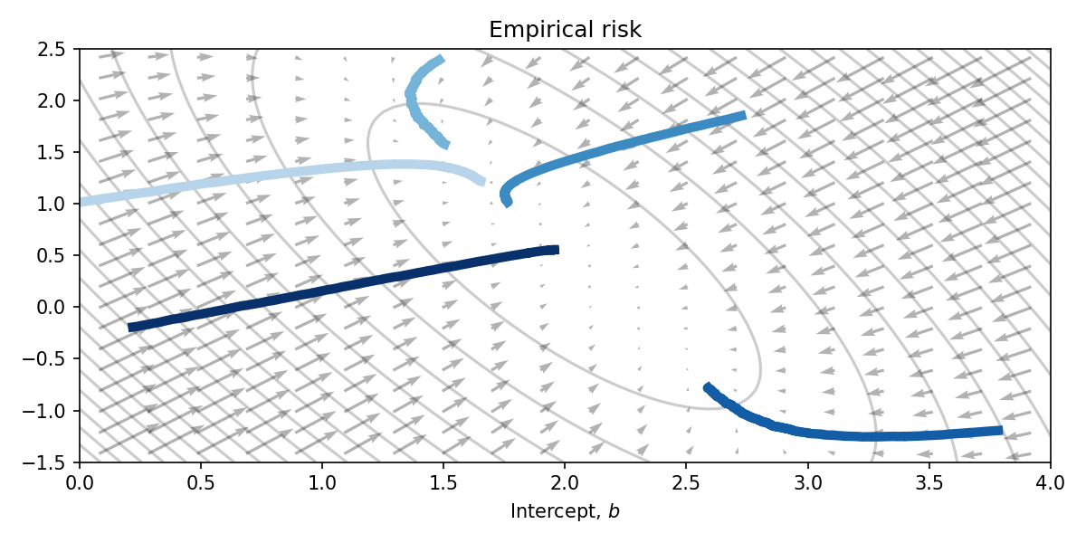
Initialising 5 different parameter values, and running each for the same duration yields the following parameter trajectories plotted on top of the empirical risk function. Clearly this is a very naive optimisation algorithm, however the parameters approach the optimum at \((2, 0.5)\) nontheless.

The direct use of JVPs in optimisation is less common. You can think of it as proposing directions in which to step (stabbing in the dark) and getting back the rate of change of \(f\) if you were to step in that direction.

Generally if \(n\), the number of inputs to our function, is large (for instance, all the parameters of a neural network) while \(m\), the number of outputs, is small (such as a scalar loss function), then using reverse-mode automatic differentiation with JVPs will be most efficient: telling us directly how much we ought to update each parameter relative to one another.

Conversely, if \(n\) was small and \(m\) was large, which is less common in machine learning, then it would be more efficient to use forward-mode automatic differentiation with VJPs.

Note that while we could compute the update procedure \(\theta_{t+1} = \theta_{t} - \eta \rvu^{\top}\rmJ\) by fully realising the Jacobian matrix, for large neural network layers this would consume unnecessarily large amounts of memory. Indeed, it is rare to ever require the Jacobian on its own, and the VJP (and JVP) allows us to avoid ever needing to store this full matrix on its own.

Returning to the linearisation view (1st-order Taylor series expansion), we can see that the Jacobian merely gives us a tangent line to our objective function. While this might be useful to determine the direction in which we should update the parameters, it does not tell us by how much and quickly becomes a poor approximation to the function, for instance ignoring the curvature.

In subsequent posts, I will go over some common first-order and second-order optimisation algorithms which seek to make more judicious parameter updates at every step.