Bayesian neural network (BNN) priors have become a contentious subject lately.
In BNNs, we first pick a prior \(\P(\rvw)\) to describe the network weights, having not yet seen any data, and proceed compute the weight posterior as the data comes in \(\P(\rvw \vert \gD) = \P(\gD \vert \rvw)\P(\rvw)/\P(\gD)\).
In practice, this choice is almost always an isotropic Gaussian \(\gN(\mathbf{0}, \sigma^{2}\rmI)\), centred at 0.
If you ask most Bayesians whether this zero-mean isotropic Gaussian prior accurately reflects their beliefs about the BNN weight distribution, or whether it yields the best generalisation, or the most accurate uncertainty estimates; they would probably say no. This is somewhat troubling, and keeps Bayesians up at night.
Signs that something might be going wrong are abound: from the often worse empirical performance of BNNs compared to identical networks trained with SGD 0: not to mention, a ballooning of the computational cost in return for your worse performance. 0[0] (Heek et al., 2019), to the cold posterior effect (Wenzel et al., 2020; Aitchison, 2020) which effectively discounts the influence of the prior in return for improved performance 1: This in particular is very troubling for the Bayesian method, since if the generative model is accurate, then Bayesian inference is optimal, then and any ad-hoc changes to the posterior should harm performance, not improve it (Gelman et al., 2003). 1[1] , and several others (Papamarkou et al., 2024).
To illustrate some of these issues slightly more concretely, consider variational inference; a popular approach to approximate the intractable posterior distribution of a finite-width BNN (Blundell et al., 2015). Variational approaches minimise an objective of the form
\[\begin{equation} \gF_{\mathrm{VFE}} = \underbrace{-\E_{\Q(\rvw)}\left[\log \P(\rvy \vert \rmX, \rvw)\right]}_{\text{expected log-likelihood}} + \underbrace{\KL\left[\Q(\rvw) \Vert \P(\rvw)\right]}_{\text{complexity penalty}}. \end{equation} \]
However, Trippe et al. (2018) suggest that minimising the KL complexity penalty above—the difficulty of which is in large part determined by our choice of prior \(\P(\rvw)\)—can lead to a pathological behaviour which they term overpruning. By setting the final hidden-to-output weights of an output neuron to \(0\), we can effectively cut off the influence of all the upstream weights in the network on the output prediction, hence turning these upstream weights into parameters we are free to move around without affecting the output. For wider 2: as determined by the relative width of the hidden layers to the output 2[2] overparametrised networks, there will be more such weights available. The network can then minimise the KL term by ensuring that lots of the weights match the prior exactly, while simultaneously ensuring that the resulting hidden activations aren’t used in the output by pruning them at the last layer so as to not mess up the predictions. The result is that the active, un-pruned network may be much smaller than expected, while the pruned weights, whose only function is to keep the KL small, end up costing us lots of memory and compute to maintain. Further, Coker et al. (2022) show that, under certain conditions in wide BNNs with isotropic priors, the variational posterior predictive reverts to the prior predictive: effectively ignoring the data.
Many of the factors causing the problems listed above conspire to give a learning objective where the optimal solution is often to collapse the posterior to the prior. This is clearly bad; resulting in unnecessarily expensive and wasteful networks, with high bias which underfit the data.
Centering the Prior on the Weight Initialisation
The idea I’d like to moot in this blog post is that the weight prior should be centred at the neural network weight initialisation locations, not \(\mathbf{0}\).
While this certainly wouldn’t be a panacea to solve all the issues listed above, it might be a first step in the right direction. This idea isn’t entirely new either, having already been used to show that such an approach improves PAC-Bayes generalisation bounds (Pitas, 2020).
Why might this be a good idea? We know that the weights aren’t initialised at zero, and for the most part they don’t seem to end up around zero after training, so centring the prior at \(0\) may be ill advised.
We also know that during training, particularly as networks grow wider, the weights may not end up very far from their initialisation, and moreover the weight progression follows simple linear trajectories (Jacot et al., 2018). For instance, the video below, taken from this excellent blog post, shows the evolution of a single \(m\times m\) weight matrix during MLP training, for successively wider networks \(m \in \{10, 100, 1000\}\):
As you can see, the weight changes in the visualisation are almost imperceptible for all but the smallest \(10 \times 10\) example.
This new weight-init conditioned prior is conceptually simple: supposing we have freshly sampled a set of neural network weights \(\rvw_{0}\) according to the best practices in deep learning theory (Glorot et al., 2010; He et al., 2015), we could treat these as the mean of our prior and use \(\gN(\rvw_{0}, \mSigma_{\mathrm{prior}})\), for some prior covariance which we might simply set to \(\mSigma_{\text{prior}} \doteq \sigma_{\text{prior}}^{2}\rmI\) to keep things cheap and simple for now 3: I defer the choice of more sensible / sophisticated covariance terms to other work; there are certainly many costs and downsides to the mean-field / independence assumption, but we won’t deal with them here. 3[3] .
This prior is valid in the sense that it doesn’t make use of any of the data, however it is still odd for a prior to be random. Perhaps we ought to marginalise over that source of randomness? In this case, we’d end up back at the standard zero-mean prior. We’ll investigate these issues below.
Use in Variational Inference
Let’s drop this prior into a simple variational inference scheme. Denote the actual, vectorised neural network parameters as \(\rvw\), and the random initialisation as \(\rvw_{0}\).
Further, let \(\rmX\) be all the inputs, and \(\rvy\) all the outputs in our dataset. We will use the following model:
\[\begin{align} \P(\rvw) &= \gN(\rvw; \mathbf{0}, \sigma_{\mathrm{prior}}^2\rmI) \\ \P(\rvw_{0}) &= \gN(\rvw; \mathbf{0}, (1-\gamma^{2})\sigma^{2}_{\mathrm{prior}}\rmI) \\ \P(\rvw \vert \rvw_{0}) &= \gN(\rvw; \rvw_{0}, \gamma^{2}\sigma^{2}_{\mathrm{prior}}\rmI), \end{align} \]
where \(0 < \gamma^{2} < 1\). This gives us a prior which is conditioned on the weight initialisation, \(\P(\rvw \vert \rvw_{0})\), and we can use variational inference to learn the weight posterior \(\P(\rvw \vert \rvw_{0}, \rmX, \rvy)\).
Is this model valid, and can we simply proceed to use it in a standard VI scheme?
Theorem 2.1. Marginalising over the weight initialisation distribution, the variational objective formed using the weight-init conditioned prior \(\P(\rvw \vert \rvw_{0})\) still forms a lower-bound on the marginal likelihood.
Proof: let us denote the new ELBO as \(\gL(\rvw_{0})\), to make the initialisation-conditioning explicit—we now wish to show that this quantity indeed still lower-bounds the log marginal likelihood:
\[\begin{equation} \label{eq:cond-elbo} \log \P(\rvy \vert \rmX, \rvw_{0}) \ge \gL(\rvw_{0}). \end{equation} \]
By marginalising out the random weight initialisations, we can write the standard marginal likelihood as:
\[\log \P(\rvy \vert \rmX) = \log \int \P(\rvy \vert \rmX, \rvw_{0})\P(\rvw_{0})d\rvw_{0}. \]
Now, substituting \(\P(\rvy \vert \rmX, \rvw_{0}) \ge \exp\left(\gL(\rvw_{0})\right)\) from the inequality in Equation \(\ref{eq:cond-elbo}\), we can see that
\[\begin{align} \log \P(\rvy \vert \rmX) &\ge \log \int \exp(\gL(\rvw_{0}))\P(\rvw_{0}) d\rvw_{0} \\ &= \log \E_{\rvw_{0}}\left[\exp(\gL(\rvw_{0}))\right] \\ &\ge \E_{\rvw_{0}}\left[\gL(\rvw_{0})\right], \end{align} \]
where we have applied Jensen’s inequality on the final line.
\(\square\)
In other words, yes, by marginalising out the weight initialisation, the new prior still yields a lower bound on the model evidence.
We can further optimise the hyperparameters using this ELBO. The two main ones are the \(\gamma^{2}\) parameters, and the prior variance. To do this optimisation, we can calculate the initial weights using the reparametrisation trick:
\[\begin{equation} \rvw_{0} = \sqrt{(1 - \gamma^{2})\sigma^{2}}\boldsymbol{\xi} \end{equation} \]
where we sample \(\boldsymbol{\xi}\) once during network initialisation. We can then learn the hyperparameters of the weight initialisation distribution, \(\gamma^{2}\) and \(\sigma^{2}\) using SGD on the normal ELBO objective, by merely including them in a parameter group of our optimiser.
Some Empirical Results
Loosely inspired by the setup of (Gal et al., 2016; Trippe et al., 2018), the following plots are from a 3-layer tanh fully-connected network trained with AdamW on the Boston UCI dataset.
As a sanity check, the following RMSE results were achieved on the UCI datasets, roughly in-line with what we would expect:
| method | boston | concrete | energy | kin8nm | naval | power | protein | wine | yacht |
|---|---|---|---|---|---|---|---|---|---|
| Weight-Init Prior | 2.84 | 4.72 | 0.47 | 0.06 | 0.00 | 3.95 | 3.85 | 0.68 | 0.84 |
| Dropout (Gal et al., 2016) | 2.90 | 4.82 | 0.54 | 0.08 | 0.00 | 4.01 | 4.27 | 0.62 | 0.67 |
| DGP (Salimbeni et al., 2017) | 2.92 | 5.65 | 0.47 | 0.06 | 0.00 | 3.68 | 3.72 | 0.63 | — |
Now taking just one split of the Boston dataset, we observe the following empirical results.
Difference in KL
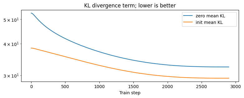
One of the motivations for using this prior, both from the PAC-Bayes theory (Pitas, 2020) and the overpruning results of Trippe et al. (2018) was that it would lead to a lower KL divergence.
Plotting the KL divergence term in the variational objective, for both a standard zero-mean isotropic Gaussian prior, and our weight-init conditioned prior shows that the KL divergence is indeed lower:
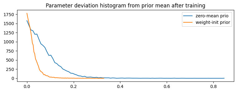
Weights Deviate Less Far From the Prior
Another property that we might expect is that, on average, the mean of the weight posterior after training is closer to the weight-init prior than the zero-mean prior. The following is a historgram 4: I’ve plotted the histogram with lines rather than bars. 4[4] showing that, indeed, the final weights tend to deviate less far from the prior when using the weight-init prior as opposed to the zero-mean prior.
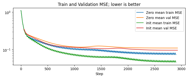
Training and Validation MSE Improves
This plot is straightforward; the MSE loss when using the weight-init conditioned prior is consistently lower than when using the zero-mean prior. The difference is larger between the training MSE lines 5: the wiggles in the training lines are due to the minibatches; the validation points are averaged across all mini-batches 5[5] than it is for the validation MSE lines, yet it is maintained nonetheless.
Effect on the Cold Posterior Effect
Finally, we can have a go at tempering the posterior (Aitchison, 2020),
\[\begin{equation} \log \P_{\text{tempered}}(\rvw \vert \rmX, \rvy) = \frac{1}{\lambda} \log \P(\rmX, \rvy \vert \rvw) + \log \P(\rvw) + \text{const}, \end{equation} \]
which, when used in the VI scheme reduces to discounting the effect of the KL
\[\begin{equation} \gL = \E_{\Q(\rvw)}\left[\log\P(\rmX, \rvy \vert \rvw)\right] - \lambda \KL\left[\Q(\rvw) \Vert \P(\rvw)\right]. \end{equation} \]
Setting different values of \(\lambda\) (denoted t in the legend below) yields:
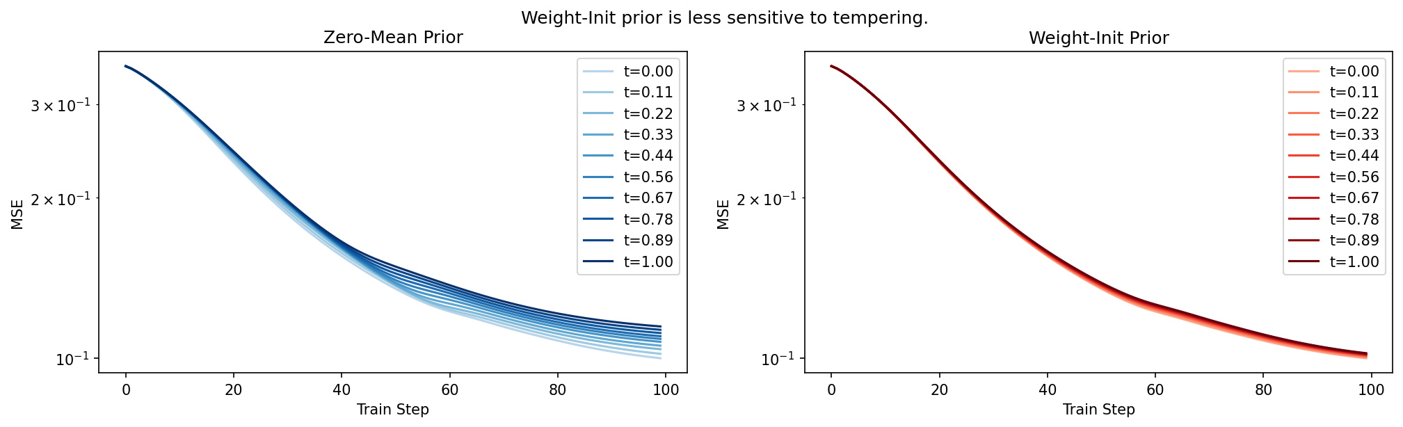
Perhaps the above isn’t surprising; if the KL term is smaller to begin with (relative to the variational log-likelihood term), then scaling it up and down should have a less pronounced effect.
Discussion
At risk of painting an overly optimistic picture with the above, it turns out that this prior is not in fact very effective.
To see why, consider that the effectiveness of this scheme depends on selecting just the right prior variance. If it is too broad, then any benefits from the non-zero prior disappear as the effect of the prior is dominated by its scale rather than its location. On the other hand if we make it very narrow, then the KL term can be driven to be very small indeed, however this comes at the cost of using a needlessly restrictive prior, which applies extremely strong regularisation towards the network initialisation, and hurts performance.
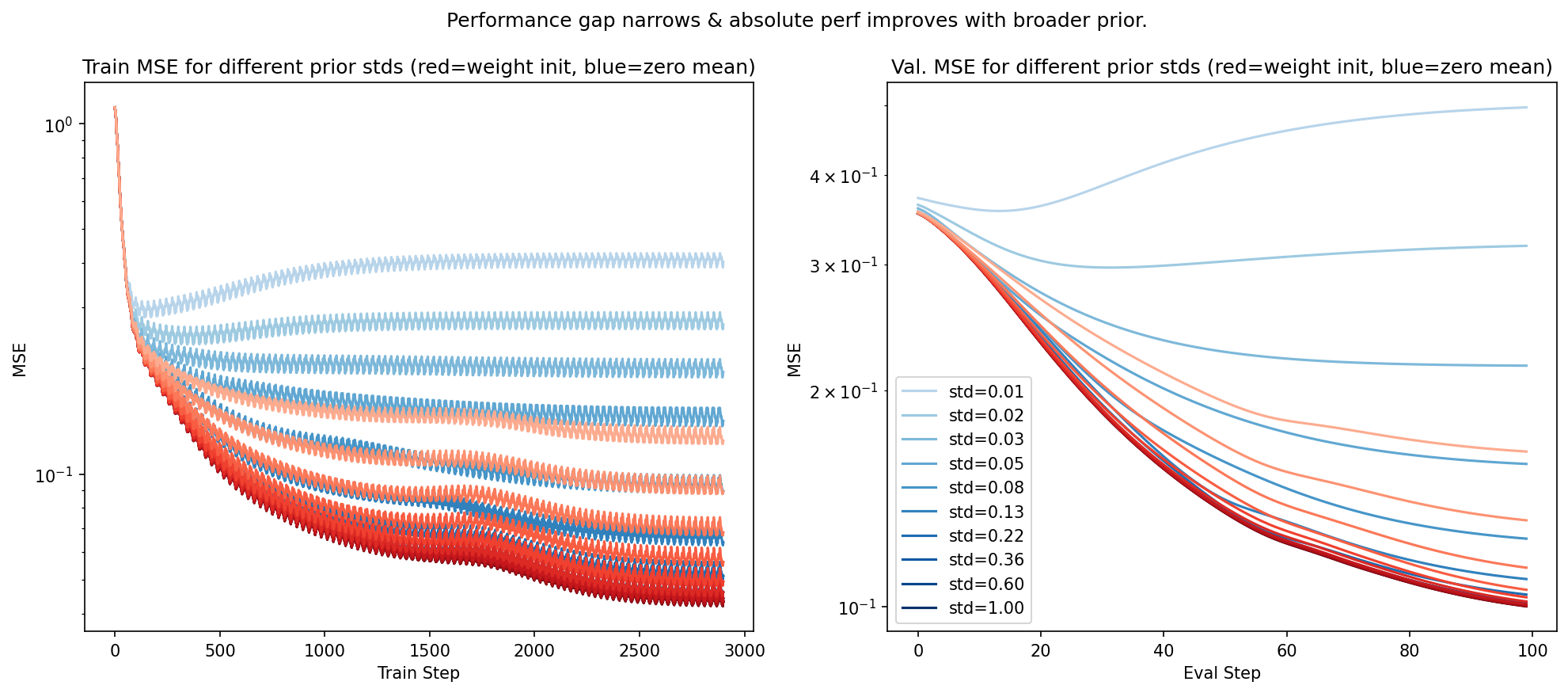
The plot below shows the effect of varying the prior variance: lighter lines correspond to a narrower prior, while darker lines correspond to a broader / less informative prior. The red lines are for the weight-init conditioned prior, while the blue lines are for the normal zero-mean prior.
As you can see, while the absolute performance, measured in MSE, of the weight-init prior is generally better than the zero mean prior, we can fairly directly control the size of the advantage by modulating the prior standard deviation. A smaller prior variance corresponds to an advantage at the cost of worse absolute MSE performance, and severely underestimated predictive uncertainty (not plotted).
With a very narrow prior centred at a given network initialisation, one might merely view this scheme as a single element of an ensemble—it would be vastly simpler, and probably less costly, to just use a deep ensemble (Lakshminarayanan et al., 2017), or Monte-Carlo dropout (Gal et al., 2016) which purports to implicitly create an ensemble.
On the other hand, perhaps our heavy-handed treatment of the prior covariance—not only the independence assumption, but also the manual initialisation without much thought—is at fault. Future work may fix this by moving beyond the independence assumption, or identifying dimensions which ought to be broader or narrower as a function of the initialisation or training dynamics.
Regardless, the somewhat degenerate behaviour exhibited above leaves doubts as to whether this prior is useful at all. I would advise against using it in its current form, although with some work on the covariance it might be salvaged. Moreover, the investigation above only considered VI—other Bayesian approximations are available and there is a slim chance that using MCMC, SGLD or a Laplace approximation the results might work out differently.