When putting LLMs to use in a specific application, you might find that the model is weak on one or more tasks that matter for your use case. This might arise through testing, or customer complaints about the model failing on some edge case.
In this post, I’d like to explore some examples where it is possible to resolve this problem using an(other) LLM 0: either the same one or another LLM 0[0] to bootstrap / generate ourselves some data to rectify these shortcomings.
As a simple example, one common shortcoming of some earlier models (for instance, GPT2) was that they lacked multiple-choice symbol binding (MCSB) abilities. That’s just a fancy way of saying: the model struggled to associate the label of a multiple-choice question with the associated answer. For example, when given the prompt:
Question: What did the cat do?

a) sat on the mat
b) ate my homework
c) chirped loudly

Answer:
models such as GPT2 fail to achieve above-chance performance
1: when
filtering the logits to only consider the valid answer tokens.
1[1]
. The model
hadn’t figured out how to associate a with the answer sat on the mat, or
perhaps it hasn’t understood this format yet.
It seems like this problem should be easily fixable by just fine-tuning our LLM on some appropriately formatted multiple-choice question datasets. However, with a pre-trained language model at hand, we don’t need to find such a dataset. We can just generate our fine-tuning data. Moreover, having identified the ‘skill’ that is lacking, we can create a curriculum of increasingly complex variants to ensure robustness, either by hand or with multi-step generation.
With this motivating example in mind, here is a broader ‘framework’ for grokking a task with synthetic data:

The “Generalist LLM” could be a large, hosted or self-run language model, while the “Finetuned LLM” is our small, cheap model that we’re looking to put into production.
The following will be an opinionated guide to using various tools and methods to produce a fine-tuned model. While I will focus on cases where we are synthetically generating / bootstrapping the training data for the task at hand, the general fine-tuning approach is equally as applicable when iterating over a dataset. The methods will however undoubtedly become outdated within a few months—I will attempt to update the post as new relevant methods come to light.
Generating Synthetic Data
It’s often easier to verify the solution to a problem than to come up with the solution.
This is ostensibly because the solution gives us a set of constraints which we can work in (hence limiting a search space or establishing useful context). In a similar vein, if we start with the answer to a problem, then by leveraging the constraints and context afforded by this answer, it can be easier to generate a question with that answer, than it is to answer that question 2: Note that this relation might not always hold, and it can be useful to additionally use a larger / more capable model to do the question generation nonetheless. 2[2] .
This suggests a general approach that we can use to generate synthetic data with which to fine-tune models to learn how to do a task:
- Randomly generate / suggest / ‘brainstorm’ an answer, perhaps leveraging a large, generalist model to do so 3: although the use of an LLM at this stage is by no means necessary: any procedure to randomly generate / sample an answer for your task is suitable 3[3] .
- Generate an associated problem or question with the above answer as its solution (also using the generalist model)
- Using the model you are fine-tuning, attempt to solve the problem
- Calculate the loss between the candidate answer and the known ground-truth answer from step 1, and update the fine-tuned model’s weights accordingly.
Some loose examples of this might include generating arithmetic expressions to improve a model’s mathematical skills (Lee et al., 2023) or generating ideal responses based on a set of rules or principles to align language model output (Sun et al., 2023).
For the rest of this post, we will use with the multiple choice question answering example mentioned above.
Learning to Bind Multiple Choice Labels
As stated above, we want to teach a language model to answer multiple-choice question answering tasks by learning to associate the class label to the answer.
It turns out that this problem was fairly common among people working with smaller domain-specific language models in the past. A common solution was to resort to ‘cloze prompting’ which consists of doing a new forward pass over each of the possible answer combinations:
Question: What did the cat do? Answer: sat on the mat.
Question: What did the cat do? Answer: ate my homework
Question: What did the cat do? Answer: chirped loudly
calculating the likelihood (or perplexity) of each sentence, and normalising by the perplexity of the answer tokens alone:
Answer: sat on the mat.
Answer: ate my homework
Answer: chirped loudly
While this might be effective, this is clearly much less efficient than being able to direct output the answer label, hence we could save a lot of running costs by teaching the model this ‘skill’.
See Robinson et al. (2023) for a good overview of
multiple-chioce question answering with LLMs.
This cloze prompting approach is often a slower and more computationally
expensive way of answering multiple-choice questions with a language
model
4: Although it can allow smaller, cheaper models to answer questions
where they previously couldn’t, so this distinction is less obvious.
4[4]
—if we
had learned the MCSB skill, we could just generate a single token to
output the answer label (a, b or c in the example above) which is much
faster.
Generating MCSB Examples
To generate synthetic data for the MCSB task, we will use the following procedure, following the general framework set out above:
- We pick a list of 5 nouns at random, selecting one at random to be the ‘answer’
- We use a generalist model to generate a description of the answer word
- Ask the model we are fine-tuning which of the 5 words best matches the description
- Update the fine-tuning model using the answer word’s label as the target next token to predict.
Here’s some code to do this.
1. Answer Generation For the first step, we will use the wonderwords
library and ensure that each word tokenizes to a single token for simplicity
later:
def get_new_words(
    tokenizer: PreTrainedTokenizerFast, r: RandomWord, n: int
) -> tuple[list[str], list[int]]:
    """
    Returns `n` random nouns which encode to a single token under the
    provided tokenizer.
    """
    words, word_ids = [], []

    for _ in range(n):
        while True:
            word = r.word(include_parts_of_speech=["nouns"])
            ids = tokenizer(word, add_special_tokens=False).input_ids
            if len(ids) == 1:
                words.append(word)
                word_ids.append(ids[0])
                break
    return words, word_ids
An example usage is:
>>> from wonderwords import RandomWord
>>> from transformers import AutoTokenizer

>>> tokenizer = AutoTokenizer.from_pretrained("gpt2")
>>> words, word_ids = get_new_words(tokenizer, RandomWord(), 5)
>>> print(words)

(['movement', 'ford', 'habitat', 'tie', 'size'],
 [10298, 25779, 17570, 22134, 2159])

>>> answer = words[0]  # just take 0th word as answer: we'll shuffle later
2. Question Generation From the chosen answer, we can create a multiple-choice question of the form:
Question: Return the label of the word which best matches the description.
Description: <generated_description>
A) movement
B) ford
C) habitat
D) tie
E) size
Answer (A to E):
For this, we need to generate a description for the answer, where we can use
the following few-shot example prompt
5: While this few-shot example prompt will work
well with most models, if your model has a specific prompt format (for
example Llama-2’s
format) then you
should probably use that
5[5]
description_prompt = """Write a description for each of the following wods:

Word: satisfaction
Description: This is a pleasant feeling often associated with a sense of accomplishment.

Word: nightmare
Description: An unpleasant dream that one often wakes up from with cold sweat.

Word: coordination
Description: The act of working together as a team and communicating effectively.

Word: {}
Description:"""
Here is a simple function for generating a descriptions for a batch of examples at once, assuming access to a causal language model, and a tokenizer with padding on the left (jump to this section for the model and tokenizer setup):
def generate_descriptions(word_batch: list[str], model, tokenizer):
    description_prompts = [description_prompt.format(w) for w in word_batch]
    inputs = tokenizer(
        description_prompts, return_tensors="pt", padding=True
    )

    with t.no_grad(), t.inference_mode():
        outputs = model.generate(
            **inputs, max_new_tokens=20, do_sample=True,
            temperature=0.8, pad_token_id=tokenizer.eos_token_id,
        )
    trunc_outputs = outputs[:, -20:]
    gen_descriptions = tokenizer.batch_decode(trunc_outputs)
    return gen_descriptions
Running this gives sensible descriptions
6: note, these will be truncated if longer than 20 tokens due to our choice of max_new_tokens. While this is undesirable, it doesn’t seem to cause too many issues in practice
6[6]
.
>>> descriptions = generate_descriptions([answer], model, tokenizer)
>>> print([f"{w}: {d}" for w, d in zip([answer], descriptions)])

['ford: A shallow place in a river or stream where one can cross on foot or by vehicle.']
3. Answer the Question
We can now format the question, put it to the language model we are training, and pick out the logits corresponding to the answer tokens.
random_order = torch.randperm(len(words))
question_prompt = "Return the label of the word which best matches the description.\n\n"
question_prompt += f"Description: {descriptions[0]}\n"
question_prompt += "\n".join([
        f"{chr(ord('A') + i)}) {words[j]}"
        for i, j in enumerate(random_order)
    ]
)
question_prompt += "\nAnswer (A to E):"

question_inputs = tokenizer(question_prompt, return_tensors="pt", padding=True)
outputs = model(
    **question_inputs,
    labels=question_inputs.input_ids.clone()
)
4. Update Weights
Finally, we take a gradient step on the loss, which we can obtain as the negative log likelihood of a categorical:
answer_idx = int((random_order == 0).nonzero().item())
answer_id = t.tensor([answer_idx])
dist = torch.distributions.Categorical(logits=outputs.logits[:, -1])
LL = dist.log_prob(answer_id)
loss = -LL
The following sections will provide more detail on updating the model weights,
although we still essentially just call loss.backward() and then take a step of an
optimiser which wraps the model’s parameters.
Finetuning Procedure
In what follows, we will first discuss how to set up all the model and trainer components. Then, we will look at training a model while generating the synthetic data online, and compare this to generating the synthetic training data offline which resembles a normal fine-tuning procedure. For both of these training procedures, we will use (Ada)LoRA adapters (Hu et al., 2022; Zhang et al., 2022) and low-bit 7: i.e. 8 or 4 bits 7[7] quantization (Dettmers et al., 2022) to reduce the memory requirements. We will also run the training using HuggingFace’s Accelerate library, with which we can use the DeepSpeed integration to help us scale across multiple GPUs and nodes.
With the finetuned model in hand, you will likely want to put it to use to serve requests. Here, efficiency and latency matters, so we will look at some useful post-processing steps such as quantizing the resulting model using AWQ.
Environment Setup
Before beginning, it can be useful to set one or more of the following environment variables:
export HF_HOME="${HOME}/path/to/huggingface_cache"
export HF_DATASETS_CACHE="${HOME}/path/to/huggingface_dsets"
export TRANSFORMERS_CACHE="${HOME}/path/to/huggingface_transformers"
export BITSANDBYTES_NOWELCOME=1
export PYTORCH_CUDA_ALLOC_CONF=max_split_size_mb:128
The first three help to keep track of where data is stored—without setting
these, data (model weights, datasets) will usually be stored in your ~/.cache
directory. The BITSANDBYTES_NOWELCOME one removes an annoying bitsandbytes
library banner, and PYTORCH_CUDA_ALLOC_CONF can help reduce GPU memory
fragmentation when loading large models.
You should also generate a HF Accelerate configuration file. By default,
accelerate will use the configuration under
${HF_HOME}/accelerate/default_config.yaml, but I recommend setting this to
somethign specific to this project by running the following command:
accelerate config --config_file path/to/accelerate_config.yaml
Select options according to your computing environment; I recommend using
bf16 precision, as well as DeepSpeed (Stage 2).
With this confguration setup, you can now launch your script with:
accelerate launch --config_file path/to/accelerate_config.yaml \
    my_script.py
Model Components
We will now build up the main training script. The snippets provied below will illustrate all the main components you need, however you will need to put them together yourself if you’re follwing along (i.e. writing all the boilerplate and surrounding code).
See the accompanying repository for the full training files.
Low-Rank Adaptors
First, we will set up low-rank adapters, which are a common technique to reduce the computational cost of fine-tuning, using HuggingFace’s PEFT library 8: I did, in 2022, write a small library for finetuning models with LoRA adapters, called finetuna. While I wouldn’t necessarily recommend using it since it is somewhat feature poor, it does provide a single-file implementation of LoRA if you’re interested in seeing a simple implementation. 8[8] . Low-rank adapters (LoRA) are a simple and effective way of reducing the computational and memory cost of fine-tuning models by, learning a low-rank weight matrix which is added to the pre-trained weights. That is, if \(\rvx\) is an input activation vector for a layer, \(\rmW \in \R^{d\times d}\) is the pre-trained weight vector, and \(\rvh\) are the hidden activations (i.e. outputs) of that layer, we add a low-rank matrix \(\rmB\rmA \in \R^{d\times d}\), with \(\rmA \in \R^{r\times d}\) initialised from random Gaussian samples \(\ermA_{i,j} \sim \gN(0, \sigma^{2})\) and \(\rmB \in \R^{r\times d}\) initialised to a matrix of all zeros \(\mathbf{0}\) to find the hidden activations as \(\rvh = (\rmW + \rmB\rmA)\rvx\).
To use LoRA adapters in training, we simply initialise a peft configuration
object. Here is an example; see this
description
of the common parameters for more information.
from peft import LoraConfig

lora_config  = LoraConfig(
  r: 8
  lora_alpha: 8
  target_modules: ["c_attn", "c_proj", "c_fc", "c_proj", "lm_head"]
  lora_dropout: 0.05
  bias: "none"
  task_type: "CAUSAL_LM"
  inference_mode: false
)
Note that you must modify the target_modules above to reflect the names of
the modules in your model. To inspect these layer names, you can simply print
out the nn.Module; for example, for gpt2 you can run the following in a
Python REPL
>>> from transformers import AutoModel
>>> model = AutoModel.from_pretrained("gpt2")
>>> model
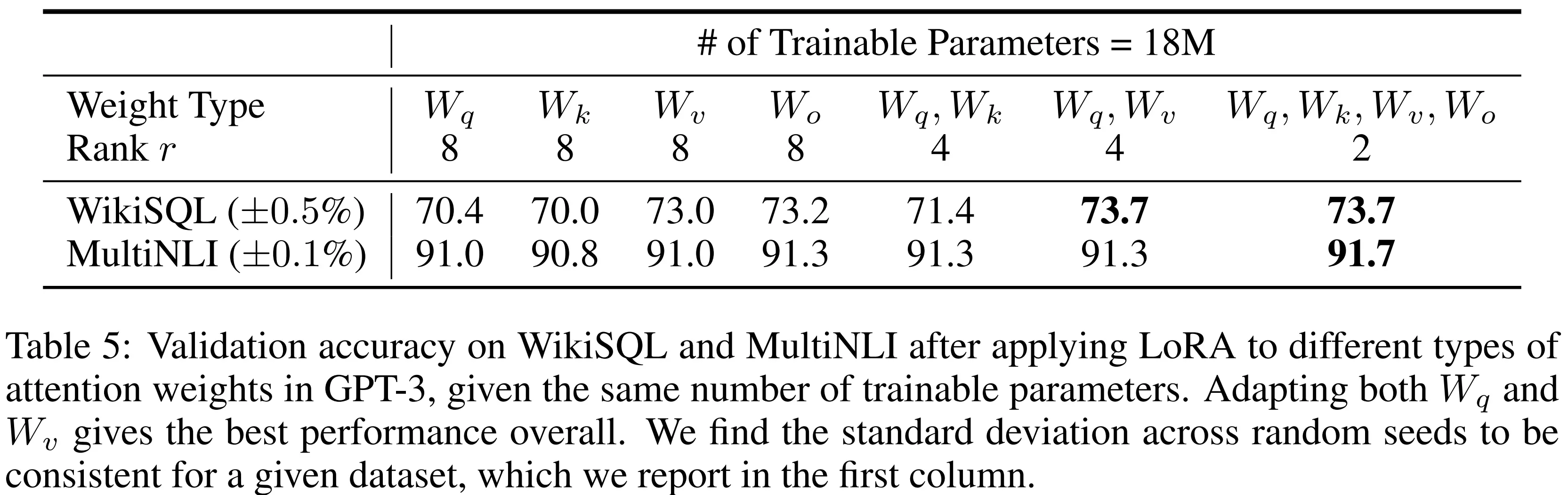
The choice of modules to adapt is up to you. From Table 5 in the original LoRA paper (Hu et al., 2022), it appears that adapting both the query and the value matrices strikes a good trade-off between performance and cost.
For a more recent method that not only automates the choice of which layers to
adapt but also adaptively varies the amount of compute/memory allocated to each
layer depending on its importance to the output, use the AdaLoRA method of
Zhang et al. (2022). This is implemented in HuggingFace’s
PEFT library, and you can trivally use it by replacing the LoraConfig
class above with AdaLoraConfig:
from peft import AdaLoraConfig

lora_config  = LoraConfig(
  lora_alpha: 8
  task_type: "CAUSAL_LM"
  inference_mode: false
)
Note that this class inherits the fields from LoraConfig, while adding some
additional
fields.
Weight Quantisation
If we are training a large model, we can often quantise the weights to a
low-bit precision (such as 8 or 4 bits) while only incurring a small hit in
model performance. Quantising the pre-trained model weights is orthogonal to
the LoRA method described above, and the two methods in fact play rather nicely
together: the frozen, pretrained weights can be stored in a low-precision
datatype, reducing the memory bandwidth required to load the model into
VRAM, while the activations and LoRA weights are kept in higher precision
(such as bfloat16 or even float32) for training.
The bitsandbytes library of
Dettmers et al. (2022)—which implements low-bit datatypes—is used
by the HuggingFace transformers, making weight quantisation as simple as
passing load_in_8bit=True or load_in_8bit=True in the
AutoModel.from_pretrained method.
There are however a few more parameters that can be configured; here is an
example of a 4bit BitsAndBytes config:
from transformers.utils.quantization_config import BitsAndBytesConfig

quant_cfg = BitsAndBytesConfig(
    load_in_4bit=True,
    load_in_8bit=False,
    llm_int8_threshold=6.0,
    llm_int8_has_fp16_weight=False,
    bnb_4bit_compute_dtype="float16",
    bnb_4bit_use_double_quant=True,
    bnb_4bit_quant_type="nf4"
)
We can also define ourselves a little helper function which will prepare a HF Transformer model for quantised training:
def prepare_model_for_quantized_training(model, use_gradient_checkpointing=True):
    is_quantized = getattr(model, "is_loaded_in_8bit", False) or \
                   getattr(model, "is_loaded_in_4bit", False)

    for name, param in model.named_parameters():
        # freeze base model's layers
        param.requires_grad = False

    # cast all non INT8 parameters to fp32
    for param in model.parameters():
        if (param.dtype == t.float16) or (param.dtype == t.bfloat16):
            param.data = param.data.to(t.float32)

    def make_inputs_require_grad(module, input, output):
        output.requires_grad_(True)

    if is_quantized and use_gradient_checkpointing:
        if hasattr(model, "enable_input_require_grads"):
            model.enable_input_require_grads()
        else:
            def make_inputs_require_grad(module, input, output):
                output.requires_grad_(True)
            model.get_input_embeddings().register_forward_hook(
                make_inputs_require_grad
            )

        # enable gradient checkpointing for memory efficiency
        model.gradient_checkpointing_enable()

    return model
Model Components and Training Machinery
What now follows is a fairly standard initialisation of the basic HuggingFace model components. We will assume the use of a decoder-only transformer (i.e. a causal language model in the HuggingFace terminology). The following initialises the model, and applies our quantization and LoRA configurations:
from peft import get_peft_model
from transformers import AutoModelForCausalLM

model_name = "gpt2"  # replace with your model's name or path
model = AutoModel.from_pretrained(
    model_name, quantization_config=quant_cfg
)
model = prepare_model_for_quantized_training(model)
model = get_peft_model
For this multiple-choice question answering task, it will be more convenient to add padding to the left so that we can simply read the final logit of each batch as the label predictions. Hence, we set up the tokenizer as follows, using the beginning of string token as the padding token:
from transformers import AutoTokenizer

tokenizer = AutoTokenizer.from_pretrained(
    model_name, padding_side="left"
)
tokenizer.add_special_tokens({"pad_token": tokenizer.bos_token})
We can also set up a PyTorch optimizer as usual:
opt = torch.optim.AdamW(
    lr= 1e-4, betas= [0.9, 0.999], eps= 1e-5, weight_decay= 0.1
)
Note that is often a good idea to include a learning rate scheduler, to ramp up the learning rate at the beginning of training, and then slowly decay it throughout the rest of training. Warmup has been shown to resolve instabilities with Adam-style optimisers, particularly during pre-training and with larger models (Liu et al., 2020). Here is an example of a simple linear scheduler:
import transformers

lr_scheduler = transformers.get_linear_schedule_with_warmup(
    optimizer=opt,
    num_warmup_steps=cfg.num_warmup_steps,
    num_training_steps=total_train_steps,
)
Accelerator
The HuggingFace accelerate library provides an Accelerator class which wraps
model components and facilitates data parallelism / multi-node training. At the
most basic level, you can simply initialise the accelerator as follows:
from accelerate import Accelerator

accelerator = Accelerator()
We now provide all the model components to this class to allow accelerate to
wrap them. Note that we don’t have a dataset, since we will be generating
synthetic data on the fly.
model, opt, lr_scheduler = accelerator.prepare(model, opt, lr_scheduler)
Online Finetuning
We can now run the main training loop, which will closely resemble the steps taken in the previous section.
Here is an online loop:
r = RandomWord()

def clean(seq: str, sep: str) -> str:
    return seq.split(sep)[0].strip() if sep in seq else seq

for it in range(num_iters):

    # Select random words
    word_lists = [
        get_new_words(tokenizer, r, 5)[0]
        for _ in range(micro_batch_size)
    ]

    # Generate descriptions for answer
    desc_prompts = [
        description_prompt.format(wl[0])
        for wl in word_lists
    ]
    inputs = tokenizer(desc_prompts, return_tensors="pt", padding=True)

    with model.disable_adapter(), t.no_grad(), t.inference_mode():
        outputs = model.generate(
            **inputs,
            max_new_tokens=20,
            do_sample=True,
            temperature=0.8,
            pad_token_id=tokenizer.eos_token_id,
        )
        trunc_outputs = outputs[:, -20:]
        gen_descriptions = tokenizer.batch_decode(trunc_outputs)
        gen_descriptions = [clean(s, tokenizer.eos_token) for s in gen_descriptions]
        gen_descriptions = [clean(s, "\n") for s in gen_descriptions]

    q_prompts, answer_idxs = [], []
    for i in range(len(word_lists)):
        random_ord = t.randperm(5)
        answer_idxs.append(int((random_ord == 0).nonzero().item()))
        q_prompt = "Return the label of the word which best matches the description.\n\n"
        q_prompt += f"Description: {gen_descriptions[i]}\n"
        q_prompt += "\n".join(
            [
                f"{chr(ord('A') + j)}) {word_lists[i][k]}"
                for (j, k) in enumerate(random_ord)
            ]
        )
        q_prompt += "\nAnswer (A to E):"
        q_prompts.append(q_prompts)

    q_inputs = tokenizer(q_prompts, return_tensors="pt", padding=True)
    outputs = model(**q_inputs)

    answer_ids = t.tensor([label_ids[a] for a in answer_idxs])
    LL = torch.distributions.Categorical(logits=outputs.logits[:, -1]).log_prob(
        answer_ids
    )
    loss = -LL.mean()

    loss = loss / gradient_accumulation_steps
    accelerator.backward(loss)

    # monitor the training accuracy
    last_logits = outputs.logits[:, -1]
    answer_logits = last_logits.gather(1, label_ids.T.expand(last_logits.size(0), -1))
    max_logit = answer_logits.argmax(-1)
    num_correct += (max_logit == torch.tensor(answer_idxs)).sum().item()

    if (it + 1)
        opt.step()
        lr_scheduler.step()  # make sure deepspeed doesn't step on opt step!
        opt.zero_grad()

        # log metrics
        # checkpoint model
Note that in the above, we use the model.disable_adapter() context manager
when generating descriptions. This allows us to bootstrap the frozen, pre-trained
model to generate the word descriptions, instead of needing to load a separate
model, which significantly reduces the memory requirements
9: it also ensures
that the model doesn’t enter feedback cycles where it learns to output
degenerate word descriptions to ‘game’ the objective.
9[9]
Running the above yields the following loss curve

As we can see, using \(5\) candidate answers, the model starts off with an accuracy of \(1/5\) indicating that its answers are no better than random chance. Within about 100 iterations, the accuracy has improved to be close to \(1\), indicating that the model has ‘grokked’ the multiple-choice symbol binding ‘skill’.
Post-procesing: efficient inference
With the fine-tuned model in hand we can now merge the LoRA adapters into the main model weights to simplify inference. This can straightforwardly be done with:
model.merge_adapter()
You can now save the model to disk using the save_pretrained method:
model.save_pretrained("path/to/model_dir")
AWQ, or activation-aware weight quantization for LLM compression and acceleration (Lin et al., 2023) is a very effective method for both reducing the memory consumption of the finetuned model and, as a result, increase inference efficiency through the reduced memory bandwidth required. See the llm-awq package, and the usage instructions.
Finally, while the HuggingFace transformer implementation is great for research
and development, it is still rather slow when it comes to inference. One very
good project with a clean API for efficient LLM inference is
vLLM.
It recently supports AWQ-quantised models, and you can load it by
pointing it to your saved model weights and passing the quantization=awq
flag.