Bayesian Flow Networks, with Code

Bayesian Flow Networks (BFNs) were recently introduced by Graves et al. (2023) as a new class of generative models / neural density estimators.

The initial exposition focused on broad motivations and presenting the framework in its full generality. In this blog post, I take the opposite approach: using a simple concrete example to gain a more mechanistic understanding of the sampling procedure and training process.

Hopefully, this will provide a clearer understanding of the framework for those who found the initial exposition broad and elusive 0: Correspondingly, I hope this might prompt connections to be made to related work by readers who are well read in this area, for instance to diffusion models or stochastic localization (Montanari, 2023) ^0[0] .

An Intuitive Overview

Suppose that we are trying to draw a convincing sample from an unknown distribution of interest; for example the distribution of cute cat images.

There is a ‘source’ which has access to lots of example cat images, and can provide us hints as we go along. We will be the ‘receiver’ of these hints:

Rather than trying to generate the sample in one go, we will take several stabs at it, collecting hints from the source as we do so.

Since we’re not sure about our sample, we’ll maintain a simple diagonal Gaussian distribution over each of the pixel values, that encodes our beliefs about what that pixel value should be. That is, each individual dimension for our belief distribution is independent—we keep a simple univariate Gaussian over each pixel value 1: for each channel, row and column of the picture ^1[1] . Let’s denote the parameters of all these Gaussians / the diagonal Gaussian as \(\vtheta\).

A BFN provides a mechanism to progressively update the parameters \(\vtheta\) of our simple belief distribution 2: for discrete data, we maintain a categorical distribution instead of a Gaussian ^2[2] over the data point \(\rvx\) we’re trying to generate, by slowly incorporating the ‘hints’ we receive about it, while also learning how to mix the values of all the dimensions of our data point.

After \(n\) steps of collecting hints from the source, updating \(\vtheta\), and mixing neighbouring pixels, by taking a sample from the final factorized Gaussian distribution over all the pixels, we should hopefully be able to get a convincing cat image.

When training a BFN, the source has access to a training dataset \(\gD = \{\rvx_{j}\}_{j=1}^{N}\) of observations from the distribution we’re interested in modelling. We repeat the procedure described above multiple times, learning how to combine neighbouring dimensions as we transition from an uninformative prior belief over the dimensions of a training point \(\rvx_{j}\) to a more precise belief over a specific \(\rvx_{j}\).

The name Bayesian flow comes from the idea of sending \(n\) (the number of ‘hints’ we collect from the source) to \(\infty\); yielding a continuous transmission process that progressively reveals information about \(\rvx_{j}\). In particular, the source smoothly alters the receiver’s beliefs for both continuous and discrete data, through a series of interleaved closed-form Bayesian belief updates and neural network forward passes.

A Slightly More Formal Overview

In a bit more detail, each ‘invocation’ of the BFN works with a single \(\rvx_{j}\) data point, and proceeds as follows:

1. A priori—with no communication having occurred between the source and receiver—the receiver might resign to placing a standard Gaussian, \(\gN(\mathbf{0}, \mathbf{1})\), or a uniform Categorical prior distribution 3: One might reasonably suggest that an empirical prior of all the datapoints \(\rvx_{\lt j}\) seen during training should be used. This turns out to be unnecessary since the first invocation of the network would largely replicate this behaviour. ^3[3] over this datapoint, if \(\rvx\) is continuous or discrete, respectively. Let \(\vtheta_{0}\) denote the parameters of this initial distribution.

2. The source maintains a ‘sender distribution’ which is controlled by an accuracy parameter \(\alpha\). Samples from this are just noisy versions of \(\rvx_{j}\): it is centred at \(\rvx_{j}\) for continuous data, or at the most likely class label for discrete data 4: where the likelihoods are Gaussian and categorical, respectively. ^4[4] . When \(\alpha = 0\), the samples are entirely uninformative, and as \(\alpha \to \infty\), samples from the sender distribution become increasingly informative; collapsing to a point mass over \(\rvx_{i}\) in the limit.

3. Both the sender and receiver have an pre-agreed accuracy schedule, \(\beta(t)\) which is a monotonically increasing function of time \(t \in [0, 1]\) 5: The accuracy parameter \(\alpha(t)\) above is the rate of change of this schedule; \(\alpha(t) = \frac{d\beta(t)}{dt}\). ^5[5] . This is used to control how much information is ‘drip fed’ to the receiver at each time step. Intuitively, the finite difference \(\alpha = \beta(t_{i}) - \beta(t_{i-1})\) quantifies how much additional information the samples from the sender distribution contain about \(\rvx_{j}\), over the receiver’s best guess about the sender distribution.

4. At each iteration (for \(i \in \{0, \ldots, n\}\) where \(n\) is usually around 10 – 100), a noisy sample of \(\rvx_{j}\) is drawn from the increasingly accurate sender distribution and sent to the receiver, which is used to update the receiver’s beliefs about \(\vtheta\), using Bayesian inference. Note that \(\vtheta\) is a continuous value in both the continuous and discrete data setting 6: representing the Gaussian’s mean, or the categorical probabilities ^6[6] , and that since each marginal of the joint over \(\rvx_{j}\) is factorised independently, these Bayesian updates are available in closed form.

5. The independently updated parameters, \(\vtheta_{i}\) at iteration \(i\) are passed to a network to be updated \(\vtheta_{i+1} = \Psi(\vtheta_{i}, t)\) which allows each dimension \(\vtheta^{(d)}\) to depend on each other dimension \(d' \in \{1, \ldots, D\} \setminus \{d\}\). Crucially, the BFN framework places no constraints on the form of \(\Psi\) so long as we can effectively condition on time, \(t\) 7: This can usually be straightforwardly achieved in most architectures by adding a time embedding to various layers ^7[7] . For instance, if \(\rvx\) is an image, then we can use a UNet. If \(\rvx\) is a string of text, we can use a transformer.

6. Finally, the quality or ‘goodness’ of the parameter update performed by the network at iteration \(i\) is evaluated as the difference (in KL) between the noisy sender distribution \(p_{S}\), with known accuracy \(\alpha_{i}\) at that step, and the receiver’s best guess about the sender distribution \(p_{R}\); that is, \(\KL[p_{S} \Vert p_{R}]\). This best guess distribution is called the ‘receiver distribution’ and is found as

\[p_{R}(\rvx_{j} \vert \vtheta_{i-1}; t, \alpha_{i}) = \int_{\rvx' \in \gX^{D}} p_{S}(\rvx_{j} \vert \rvx'; \alpha)\ p(\rvx' \vert \Psi(\vtheta, t)) d\rvx'. \]

To interpret the above, observe that the receiver knows the form of the sender distribution \(p_{S}(\cdot \mid \rvx_{j}; \alpha)\) 8: In the continuous case, this is just a Gaussian with known covariance which is a function of \(\alpha\), but unknown mean, \(\rvx\). For discrete data, this is a categorical. ^8[8] but does not know \(\rvx_{j}\). To deal with this, the receiver marginalises over all possible \(\rvx' \in \gX^{D}\), weighted by the probability given to \(\rvx'\) by the distribution obtained from the network output; \(p(\rvx' \mid \Psi(\vtheta, t))\).

We can see that depending on the accuracy level \(\alpha\), the goal of the network \(\Psi\) might be to output the parameters of a distribution that is either completely uninformative; a point mass over the data point \(\rvx_{j}\) itself; or anything in between.

During training, we repeat the above procedure for many different data points drawn from the data distribution, with the loss found as the sum of the KL divergences \(\KL[p_{S} \Vert p_{R}]\) for a variety of times \(t \in [0, 1]\). We learn the parameters of the ‘mixing network’ \(\Psi\) which effectively combine the parameters \(\vtheta\) of the simple belief distribution, in order to converge over \(n\) iterations to a distribution under which the data point \(\rvx_{j}\) is increasingly likely.

A Simple Continuous Example

Here is a simple univariate example with which to introduce the components of the BFN framework 9: The univariate example will miss out some of the key properties of BFNs, namely the factorisation of the marginals and local mixing between dimensions afforded by the network, but we will get to that in a later section. ^9[9] . We will consider the continuous case \(\gX = \R\) where \(D = 1\) (in other words \(x \in \R\)) and where the latent data-generating distribution will have the following density:

We now follow each of the steps outlined in the intuitions in the previous section.

Prior Distribution

In this univariate continuous setting, the prior distribution (which Graves et al. (2023) refer to as the input distribution), \(p_{I}(x \vert \theta)\) is just a univariate Gaussian:

\[\begin{align} \theta &\doteq \{\mu, \rho\} \\ p_{I}(x \vert \theta) &\doteq \gN(x\mid \mu, \rho^{-1}) \label{eq:input_dist}. \end{align} \]

We will simply use a standard Gaussian for this prior: setting \(\theta_{0} = \{0, 1\}\).

Note that I have deliberately chosen a multi-modal data distribution, plotted above, to avoid conflating the full data distribution with the distribution maintained by the BFN in Equation (\(\ref{eq:input_dist}\)) 10: and the output distribution we will see later ^10[10] , which is a distribution over a specific data point and imposes no Gaussianity constraint on the (marginal) distributions of the data being modelled.

For clarity of exposition, let’s pick a specific training data point now, \(x_{1} = 0.25\), that we’ll use as an example going forward:

As alluded to above, while we could use the empirical mean and variance of the training data seen thus far as the prior parameters \(\theta_{0}\), this ends up complicating the equations, and the network \(\Psi\) will largely fit this for us for small values of \(t\).

Sender Distribution

The sender distribution is merely a Gaussian, centred at our training point \(x_{1}\), with precision \(\alpha\):

\[p_{S}(y\mid x_{1}; \alpha) = \gN(y \mid x_{1}, \alpha^{-1}). \]

Hence, samples from the sender distribution are just noisy versions of \(x_{1}\) with varying levels of noise.

Accuracy Schedule

The noise in question is derived from the accuracy schedule \(\beta(t)\), which is found by requiring that the expected entropy of the input distribution decreases linearly with \(t\).

By defining \(\sigma_{1}\) to be the standard deviation of the input distribution at the final time \(t=1\) (this is set by hand as a hyperparameter), Graves et al. (2023) define the accuracy schedule for the continuous case as:

\[\begin{equation} \label{eq:accuracy_schedule} \beta(t) = \sigma_{1}^{-2t} - 1, \end{equation} \]

with its derivative, the accuracy rate, being

\[\begin{align} \alpha(t) &= \frac{d(\sigma_{1}^{-2t} - 1)}{dt}\nonumber \\ &= \frac{2\ln \sigma_{1}}{\sigma_{1}^{2t}}. \end{align} \]

Plotting this out for \(\sigma_{1} = 0.02\) gives the following accuracy schedule:

Note that this is undefined at \(t=0\), where we resolve to manually set \(\beta(0) \doteq 0\).

Bayesian Updates

We now come to the Bayesian updates, where we update the receiver’s belief about the data point at hand \(x_{1}\) in light of ‘hints’ received from the sender. Remember that this is initially a standard Gaussian prior, \(p_{I}(x\mid \theta) = \gN(\rvx\mid \mu, \rho^{-1})\) with \(\theta = \{\mu, \rho\} = \{0, 1\}\). The update is performed using a noisy sample from the sender distribution \(y \sim \gN(y\mid x_{1}, \alpha^{-1})\).

Crucially, since both the input and sender distributions are Gaussian, we may write the Bayesian update in closed form 11: see my previous article on the Gaussian ^11[11] as:

\[\begin{align} \rho_{i} &= \rho_{i-1} + \alpha,\\ \mu_{i} &= \frac{\mu_{i-1}\rho_{i-1} + y\alpha}{\rho_{i}} \end{align} \]

Let’s visualise these updates to the receiver’s beliefs. Below is a plot of the Gaussian prior distribution in black (which looks unusually broad due to the scaling of the plot; it is however just a standard normal distribution), in which we include the sampled data point \(x_{j}\) and the (latent) data distribution for context:

Next, we take the first sample from the sender distribution (dotted blue line), centred at \(x_1 = 0.25\), and with accuracy \(\alpha = 2\). We perform a Bayesian update on the mean in light of this stochastic sample, while performing a smooth, predictable update to the variance according to the accuracy used. The resulting updated belief is the Gaussian plotted in the solid blue line:

Continuing in this way for two more steps, we can see how the sender distributions (dotted lines) become increasingly accurate and hence the samples (vertical lines) increasingly informative about \(x_{j}\). Correspondingly, the receiver’s beliefs about the data point at hand (solid lines) become increasingly accurate:

It turns out that since the noise schedule is known, we may obtain the posterior over the parameters \(\theta\) at any given time conditioned on a data point \(x_{1}\) in closed form as:

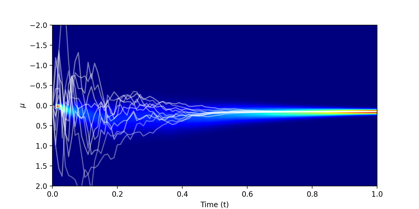
\[\begin{equation} \label{eq:bayesian_flow_dist} p_{F}(\theta\mid x_{1}; t) = \gN\big(\mu \mid \gamma(t)x_{1}, \gamma(t)(1-\gamma(t))\big), \end{equation} \]

where

\[\begin{equation} \label{eq:gamma} \gamma(t) \doteq 1 - \sigma_{1}^{2t}. \end{equation} \]

The authors refer to this as the Bayesian flow distribution. Below is a visualisation of this Bayesian flow distribution, for our data point \(x_1 = 0.25\), with \(\sigma = 0.01\) and \(100\) timesteps. The trajectories all begin at \(\mu_{0} = 0\), before fanning out and eventually converging on \(\mu = 0.25\).

Network Forward Pass

We now come to the point where we apply the network \(\Psi\) to mix information from the different dimensions of the data / ‘attend’ to different parts of the data point.

Admittedly, the virtues of this inter-dimension mixing step are somewhat lost on our one-dimensional toy example. This doesn’t prevent us from proceeding nonetheless.

Taking inspiration from diffusion models (Ho et al., 2020), rather than outputting the updated parameters directly \(\theta_{i} = \Psi(\theta_{i-1}, t)\), Graves et al. (2023) predict a Gaussian noise vector \(\epsilon \sim \gN(0, 1)\) that was used to generate the mean passed as input to the network 12: Recall, the only parameter we learn in the continuous setting is the location of the Gaussian belief over \(x_1\) ^12[12] .

From Equation (\(\ref{eq:bayesian_flow_dist}\)) above, we had that

\[\mu \sim \gN\big(\gamma(t)x_{1}, \gamma(t)(1-\gamma(t))\big). \]

Reparametrising,

\[\begin{align*} \mu &= \gamma(t)x_{1} + \sqrt{\gamma(t)(1-\gamma(t))}\epsilon \\ \implies x_{1} &= \frac{\mu}{\gamma(t)} - \sqrt{\frac{1-\gamma(t)}{\gamma(t)}}\epsilon. \end{align*} \]

Thus the network outputs an estimate \(\hat{\epsilon}(\theta, t)\) of \(\epsilon\), and we can transform this into an estimate of the data point \(\hat{x}_{1}(\theta, t)\) with

\[\hat{x}_{1}(\theta, t) = \frac{\mu}{\gamma(t)} - \sqrt{\frac{1-\gamma(t)}{\gamma(t)}}\hat{\epsilon}(\theta, t). \]

As with the accuracy schedule, note that at time \(t=0\) the output is undefined due to \(\gamma(0) = 0\). We resolve to set \(\hat{x}_{1}(\theta, t) \doteq 0\).

Training Loss

Omitting derivations, the continuous-time loss from the full framework (i.e. for use in both the continuous and discrete data case) is:

\[L^{\infty}(x) = \lim_{\epsilon \to 0}\frac{1}{\epsilon} \E_{t\sim U[\epsilon, 1],\ p_{F}(\theta\vert x, t-\epsilon)}\left[\KL\big[p_{S}(y \mid x; \alpha(t, \epsilon)) \Vert p_{R}(y \mid \theta; t-\epsilon, \alpha(t, \epsilon))\big]\right] \]

The continuous-time loss simplifies quite a bit for the continuous data case, resulting in

\[L^{\infty}(x) = -\ln \sigma_{1}\E_{t\sim U[0, 1],\ p_{F}(\theta\vert x; t)}\left[\frac{\Vert x - \hat{x}(\theta, t)\Vert^{2}}{\sigma_{1}^{2t}}\right]. \]

Example in PyTorch

Here is an example of fitting our example univariate data using the associated torch_bfn package in my accompanying repo.

We begin with some imports

import torch as t
import torch_bfn

and creating a dataset from the simple multi-modal data distribution we have been using throughout:

from torch.distributions import Categorical, Normal, MixtureSameFamily

mixture_weights = t.tensor([0.4, 0.6])
means = t.tensor([-0.3, 0.2])
stddevs = t.tensor([0.1, 0.07])

categorical = Categorical(mixture_weights)
component_distribution = Normal(means, stddevs)
data_dist = MixtureSameFamily(categorical, component_distribution)

train_x = data_dist.sample((1000,1))
train_x, denorm = norm_denorm(train_x)
train_loader = DataLoader(TensorDataset(train_x), batch_size=128)

We initialise a suitable network for \(\Psi(\theta, t)\): here we’ll use a simple residual network with linear layers and sinusoidal time embeddings, which I provide in the library:

net = torch_bfn.LinearNetwork(dim=1, hidden_dims=[64, 64])

We can now initialise the continuous Bayesian flow network class as follows:

bfn = torch_bfn.ContinuousBFN(dim=1, net=net)

Our training loop looks as follows, where we have an EMA utility which computes an exponential moving average of the model’s parameters.

opt = t.optim.AdamW(bfn.parameters(), lr=1e-3)
ema = torch_bfn.EMA(0.9)
ema.register(bfn)

for i in range(1000):
    for batch in train_loader:
        X = batch[0]
        loss = bfn.loss(X, sigma_1=0.01).mean()
        opt.zero_grad()
        loss.backward()
        t.nn.utils.clip_grad_norm_(bfn.parameters(), 1.0)
        opt.step()
        ema.update(bfn)

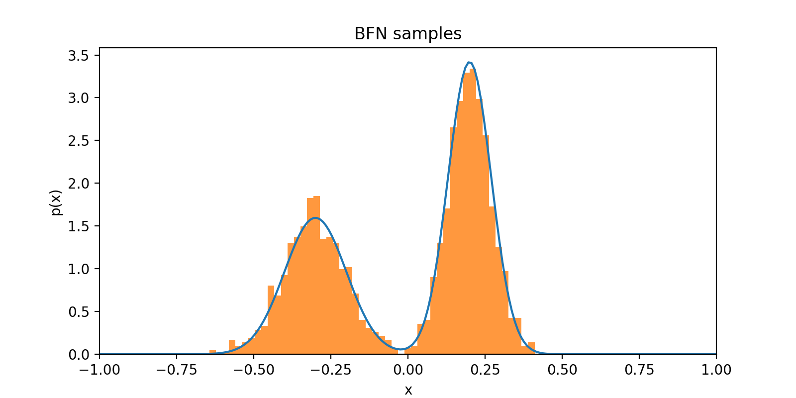
Finally, we can draw some samples to see how we did

samples = bfn.sample(n_samples=1000, sigma_1=0.02, n_timesteps=10)

Practical Tips

Here is some anecdata from my implementation:

• It seems important to normalise each of the dimensions to lie within \([-1, 1]\). This should not be an issue unless your data will be heavily nonstationary.

• Using an exponential moving average of the network weights during training seems to stabilise things a lot.

• Try varying \(\sigma_{1}\) and \(n\) (the number of time steps) to get good samples—as you decrease \(\sigma_{1}\), increase \(n\). Generally \(\sigma_{1} = 0.01\), \(n = 10\) is a good place to start, and you might end up at \(\sigma_{1} = 0.00001\), \(n = 100\).

• Generally, there seems to be a trade off with the size of \(\sigma_{1}\) and the number of sampling steps. You can get very fast sampling by tuning \(\sigma_{1}\) to a fairly large value with \(n \approx 10\). However the outcome is very sensitive to using the right hyperparameters. To get a sampling procedure that is more robust to the hyperparameter setting, you can turn down \(\sigma_{1}\) and increase \(n\) to something between \(50\) and \(100\), however this obviously comes at the cost of slower sampling.